Calculating Correlation Coefficients with Oracle Analytics CORN function

Oracle Analytics platform provides multiple functions to analyze and better understand your data. This blog explains a prebuilt function that makes it very simple to calculate Pearson's Correlation Coefficient (PCC) between two columns. This function is called CORN in Oracle Analytics. Before going any further let us remember what correlation coefficient is and what it is used for.

What is correlation coefficient?

Correlation coefficients are used to measure the strength of relationship is between two metrics. Pearson’s correlation coefficient (PCC) is commonly used for statistical analysis. The correlation coefficient ranges from -1 to +1. The meaning of this value is:

• When the coefficient is 1, it means the metrics are perfectly correlated to each other.
• When the coefficient is -1, it means the metrics are inversely correlated to each other.
• When the coefficient is 0, it means the metrics are not correlated to each other.

The formula for calculating PCC between two columns X, Y with n data points is as follows.

Note an implicit yet aspect of this expression : the grain of the data, ie what each individual record represents. Implicit is, that X Y data pairs are available at the level needed for the analysis. For example : correlation between car weight (X) and avg fuel consumption (Y), is implicitly meant 'by car'. Input data is typically distinct weight and fuel consumption for each car in a population of N cars. The grain of the data here, is car level.

But perhaps that same analysis is meaningful as well at a different level : by car makers maybe, or by type of fuel, or by type of engine... Changing the grain means to provide the input data at an aggregated level for the new grain. If we wanted correlation of X and Y by car manufacturer, we would need to average, for any given car maker, the weight of every cars he produced as well as the avg fuel consumption for that same group. That, would become the input data to our correlation function.

Understanding CORN Function

So now, let us take a look at the CORN function in Oracle Analytics and understand its components.

CORN function syntax requires 3 parameters as follows:

CORN(Metric1, Metric2 AtGrain(Attribute) )

• Two Metrics – Metrics for which the correlation coefficient has to be calculated
• One Attribute – the grain of the data at which the correlation is calculated

The CORN function does not take any implicit decision, and hence will expect from the user that he specifies the grain he expects the computation for. If employees data in a database is at the employee level (one row for each employee), the CORN function will require user to specify what level it should compute by. For example, if user specifies Department, the function will automatically aggregate the metrics X and Y by department first, then calculate the correlation on the resultset at that level.

Let's say we are analyzing correlation between two employee columns “AGE” and “JOBSATISFACTION” , but we want it at “DEPARTMENT” level grain. Go to My Calculations :

Add function to the calculation: CORN(AGE, JOBSATISFACTION AtGrain(DEPARTMENT) ) 

Visualize the value in Canvas

Example (Grain @ Row ID)

There are instances when you user may want the grain level to be each row from the dataset. If a row level identifier exists for the dataset, then that's to be used in the AtGrain condition. If unique identifier does not exist, then create one using Rowid() function as show in the following blog : Unique ID Creation

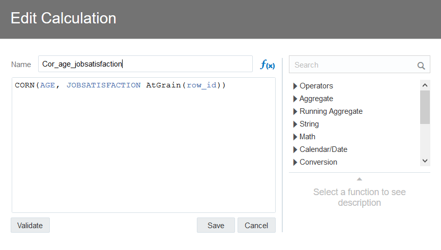
Once we have that we can replicate the CORN  function at ROW_ID level. Go to My Calculations and apply function : CORN(AGE, JOBSATISFACTION AtGrain(ROW_ID) )

You can view the correlation value at ROW_ID level.

Drag and drop the column on the canvas to see the calculated value. Once the calculation is on canvas, you can filter by one of the attributes and observe how the metrics are correlated for that selection.

CORN function is useful and handy for understanding the relationship between metrics in depth and help you understand the relationship between columns better.

If you need to apply this function to a matrix of different metrics columns at once, then use the correlation matrix vanilla visualization. This Viz will provide you with a heatmap matrix with correlation values for each intersections in your matrix. 

Note that in this case, the grain of the calculation is defined by setting an argument in the Detail field, on the viz grammar pane.

Thanks for reading the blog!

 

 

Consuming Analysis from Spatial Studio directly from OAC

Spatial Analysis is a process in which you model problems geographically and compute results using various spatial calculation. This is something that is used widely in many scenarios which include analyzing the results of an election, finding areas that are likely to affected by a hurricane when it makes a landfall, etc... Spatial technology helps in understanding where things occur, measuring sizes, shapes, geographical distributions, relationships and interactions between places, and more.

Spatial Studio is a web application built by Oracle that provides a great graphical user interface leveraging the underlying Oracle Database spatial functions. Once Spatial calculations and analysis are computed with Spatial Studio, results can then easily be dynamically visualized in Oracle Analytics. This blog shows how to enable that dynamic aspect of consumption of Spatial Studio analysis directly into Oracle Analytics.

In our scenario here, we work at an insurance company in the United States with many home or car insurance customer policies. US meteorological department just predicted that hurricane NATE will be making a landfall in the country in another couple of days. Experts are predicting that it will create havoc to real estate assets that lie within the 100 kms buffer of it's path. As a business analyst for the insurance company, we need to analyze and asses the likely damage to the properties and the expected expenditure. This is a perfect example for spatial analysis and we are going to see how Spatial Studio in combination with OAC is making it very easy for us. 

The first step is to proceed with the spatial analysis in Spatial Studio 

Let's upload the customer assets data into Studio (the database) as well as the geographical data associated with the hurricane expected path. The data for the hurricane was obtained under the form of shape files (from the web). Visualizing these two overlaid onto each other in Spatial studio renders this :

Then, Studio easily allows to compute and visualize a buffer of 100kms around the hurricane path. This can be done by using the transform operation in studio to add a buffer of 100kms distance. 

Finally we a spatial analysis will identify all the customer assets that lie inside the buffer zone. This is achieved by the usage of the Filter operation that returns all shapes contained inside another.

That was so easy and the resulting spatial analysis is now saved into the Spatial Studio database. Le'ts just go and check the list of datasets in the Spatial Studio, where we should find the results of our analysis.

Let's now expose the Spatial calculations results directly to Oracle Analytics

With its 20.1 release, Spatial Studio now allows to represent these results under the form of a query-able synonym object in the database. Right click on a spatial analysis dataset and choose Properties. Under the Settings tab, a new property field called "Synonym" is introduced. Give a name that you want to assign to the spatial analysis dataset to this field. This will be the name of the public view in which the spatial analysis dataset will be saved in the database. In this example, let us give it a name 'oac_spatial_analysis' and choose Apply.

So at this point, we completed the analysis in Studio to identify customer assets that are at risk because of the hurricane, and we have assigned a synonym value to the results-set of this data. The work Spatial Studio part is now completed and let us move on to the OAC part.

From an OAC instance, let's create a connection to the database used by Spatial Studio and choose the appropriate schema. Now search for the synonym name to find the corresponding spatial analysis dataset. In our case, we search for 'oac_spatial_analysis'.

We can see the dataset, but we cannot directly add it into OAC since it contains columns of SDO_GEOMETRY data type. As of 5.9 release, OAC cannot handle that datatype but it will be enabled soon in an upcoming release. Meanwhile, the temporary workaround for adding spatial analysis dataset is be to enter a SQL command to get all the data from the spatial analysis dataset except for the SDO_GEOMETRY column :

In the above picture, we have issued a SQL statement against oac_spatial_analysis (synonym) view which includes all the columns except for the geometry column. This includes valuable information such as customer ids, names, addresses etc. We can now add this dataset into OAC.

Now we can visualize the list of customer assets that are at risk and the business analyst of the insurance company can get quick insights by blending this spatial results with his onw business datasets in OAC.

Thanks for reading this blog !

Oracle Essbase 21.1 is Available

If you’ve been using Essbase standalone (11g) for years, and yearning for the day that you could take advantage of the latest Essbase features, but remain on your independent, standalone Linux platform, THAT DAY IS HERE!

We’re excited to announce the availability of Essbase 21c. This new release has many enhancements of the Essbase features you’ve come to know and value. It also gives you all the latest features available in our Essbase 19c cloud offering, PLUS! it enables you to continue to work from your standalone, Linux platform.

You can download Essbase 21c on Oracle Software Delivery Cloud. For details on platform support and certification matrix, see our External MOS certifications. For those of you looking forward to Essbase 21c for the Microsoft Windows platform or the upgraded Essbase 21c on Oracle Cloud Infrastructure Marketplace, those will follow in just a few months. Stay tuned.

Oracle Essbase is a business analytics solution that uses a proven, flexible, best-in-class architecture for analysis, reporting, and collaboration. Oracle Essbase delivers instant value and greater productivity for your business users, analysts, modelers, and decision-makers, across all lines of business within your organization.

New features in 21c

Essbase 21.1 comes with its own installer and configuration tools. As noted, you get all the new features we’ve introduced on the cloud, as well as in 19c. Some notable new features include – a modern browser-based UI for management and administration, Cube Designer plug-in for Smart View, platform features like Connections/Datasources, new security roles, dynamic filters and more.

Why 21c?

With 21c, you get the choice of an independent Essbase install with the latest product features and platform support. Existing customers can easily migrate their 11g applications to 21c using the LCM migration utilities. New client utilities and REST APIs enable customers to develop custom analytic solutions.

Here are more resource for further details on the release

Check New Features in the Doc

New features and overview of 21c (Videos)

Release Notes

Differences between 11g and 21c

Migration to 21c 

Thanks for your interest with that blog !

OAC querying JSON Data with AJD (Autonomous JSON Database)

JSON or JavaScript Object Notation is an open data format and the preferred data interchange format for web applications. JSON format is highly used in developing web applications where fast, compact and convenient serialization of data is required.

While Oracle Analytics Cloud (OAC) does not inherently support JSON format data sources, overcoming this limitation is simply done by integrating with Oracle Autonomous Data Warehouse (ADW) or Oracle Autonomous JSON Database (AJD). Oracle AJD stores JSON documents in a native tree-oriented binary format and provides native, open-source document store API called SODA (Simple Oracle Document Access) that allows users to store and query JSON documents.

This short playlist gives a quick video tour of the steps involved to query JSON from OAC : OAC querying JSON data with AJD (Autonomous JSON Database)

In this blog, we will cover the steps involved in starting from a simple JSON document and enabling to visualize it directly in Oracle Analytics. An important point to note is that this should all be achieved without the user having to know any of the data architecture in the JSON... That is, I bring a JSON file which I am not familiar with, and I need to visualize it in OAC without having to understand it's structure beforehand.

Sample JSON document

Let us consider a sample JSON file with around 2000 Purchase Orders data rows. Each Purchase Order object contains several attributes like PONumber, Reference, Requestor, User, CostCenter and so on. It also has a nested array of LineItem objects. Each LineItem has attributes like ItemNumber, Part, Quantity and so on. Let's pretend we are not familiar with any of these details. For us, this is a PO Dataset :

In order to store this document in AJD (ADW), we need to make sure that the JSON format adheres to the following 'classic' specifications:

1. Each JSON object appears as a single line in the file. Attributes and nested array of objects within an object should not be on separate lines
2. Each JSON object be enclosed within curly braces 
3. No comma separator between JSON objects
4. No square brackets at the start and end of the JSON document

Here’s an example of a JSON file with the right format.

Once our format is checked, we need to go through a sequence of steps to make this JSON exist in the database, and query it with OAC.

While the list seems long, it's a series of basic steps, most of which need to be initiated only once for initial loading/analysis of the file. Subsequent refreshes of data for the same file require less steps to complete. Let’s look at each of these steps in detail :

Step 1 – Upload JSON file on OCI storage

First in the process is to upload our purchase order JSON file into an OCI object storage so it can be accessed by AJD. In order to do that, we log into to our cloud console, select Object Storage and choose an appropriate Bucket.  

Select the Purchase_order.json file from your local machine and upload it to the object store. Once the file is uploaded, choose the menu option on the uploaded file and View Object Details. This will display the URL path to access the file. Copy this path and save it for later use.

Step 2 – Create a Collection object in the Database

Next step is to connect to the AJD instance (via a SQL interface) and use SODA APIs command to create a 'collection' object that will store the JSON document. For example, connect to the database instance using SQL Developer, ensure that the user account used to make the connection is granted the database role SODA_APP, and run the following command :

DECLARE

    collection  SODA_Collection_T;

BEGIN

    collection := DBMS_SODA.create_collection('DEMO_JSON_PO');  

END;

This creates a collection called DEMO_JSON_PO. Once the collection is created, a corresponding table with the collection name is automatically created as well in the database.

Step 3 – Store JSON in the collection

Now,  you can to store the JSON document from object storage into the collection we just created. Make sure you first have a DB credential that can access the file in the object storage, to confirm that you can use the following syntax :

SET DEFINE OFF
BEGIN
  DBMS_CLOUD.CREATE_CREDENTIAL(
    credential_name => 'DEMO_CRED',
    username => 'oracleidentitycloudservice/demo.user@oracle.com',
    password => '************'
  );
END;

The username/password used in the credential creation should be one that has access to the JSON file on object storage. Once the credential is created, we use it to copy the JSON document into the collection using the following syntax

BEGIN 
 DBMS_CLOUD.COPY_COLLECTION(   
    collection_name => 'DEMO_JSON_PO',
    credential_name => 'DEMO_CRED',
    file_uri_list   =>
      'https://objectstorage.us-ashburn-1.oraclecloud.com/n/xxxxxxxxxxx/b/oacdemostorage/o/purchase_order.json',     
    format          =>
      JSON_OBJECT('recorddelimiter' value '''\n''')  );
END;

In the syntax, use the collection and credential name created in the above steps. file_uri_list is the URL to the JSON file on object storage (stored in step 1) . Recorddelimiter is a newline character in our JSON file.

Once the copy_collection is executed, we can confirm things by query the DEMO_JSON_PO table in the database and we find that each JSON line from the source file is loaded as a separate row in this table. The JSON contents are loaded into a blob column called json_document. 

Step 4- Create JSON index

Now that we’ve stored the JSON data in the collection, next step is to flatten this JSON structure into rows and columns so we can query it from OAC. Keep in mind we don't know the architecture of our JSON data hierarchy. So in order to do this flatting without this information, we first create a search index on the json column using the following syntax

Create search index DEMO_JSON_PO_IDX on DEMO_JSON_PO (JSON_DOCUMENT) for JSON parameters ('DATAGUIDE ON') ;

Here DEMO_JSON_PO_IDX is the index name, DEMO_JSON_PO is the collection name and JSON_DOCUMENT is the blob column name.  Specifying ‘DATAGUIDE ON’ is important in order to be able to extract the JSON schema as columns. This is actually what will parse the JSON file architecture into a series of flattened columns for us. Creating this search index will result in the creation of a set of related DR$ tables.

Step 5- Flatten JSON into relational format

Finally, we create a Database view with expanded columns for the tree structure of the JSON using the following syntax

exec dbms_json.create_view_on_path ('DEMO_JSON_PO_FLAT','DEMO_JSON_PO','json_document','$');

where DEMO_JSON_PO_FLAT is view-name, DEMO_JSON_PO is the collection name, json_document is the column with blob and $ indicates JSON path from the root. On executing this procedure a Database view is created with the JSON schema extracted as distinct columns. And each JSON object (line from our original file) is extracted as one or more rows in this view.

Step 6 – Query flattened data in OAC

That's it, we are done with flattening this JSON Data ! We can now simply query it via SQL commands. So to make it available in OAC we just need to create it as a dataset in OAC. One caveat, as the column names in the view are of the format JSON_DOCUMENT$xxx, previewing a dataset that is directly sourced from this view in OAC will likely result in “Invalid identifier” error. To get around this we just need to click the 'Enter SQL' option during dataset creation, just after we select all the columns of the view. Here, for each column specify an alias column name. 

At this point, we are able to query this flattened view directly from OAC retrieve data and visualize like any other source ! This datasource can be used in connection with any other OAC source, and for any of the OAC capabilities (dataviz, data flows, ML, Mobile, Answers...)

Incremental Data Refresh Scenario

Previous section described the various steps required for an initial load of JSON document into an AJD collection. For subsequent refreshes only a subset of these steps  are involved : 

- For simple JSON data refresh with no changes to JSON structure, following are the steps to follow

- For JSON data refresh with changes to JSON structure, following are the steps to follow

Thanks for your time reading this blog !

Easily Get a Unique ID Column in Your OA Dataset

It often happens to me that, while analyzing data, I end-up needing a unique identifier for every row in my dataset, but... it's just not present in there.... Doesn't that happen to you too sometimes ? Whether the underlying data is self uploaded , or is an enterprise semantic layer, sometimes simply we don't have the choice to go back to the physical data and add a unique row id for each record in the data. Yet there are cases where we badly need that info : for some specific visualizations (Box-plots, Scatter-plots, etc...), or to set an aggregation level for a calculation for example. 

How do you resolve this easily if you don't have access to the underlying physical data ? Here is a very simple way to address this with a small Oracle Analytics calculation, which is not intrusive to the underlying data-source : the 'Rowid()' logical function.

The video just below gives a quick tour of how to use Rowid()

There is an easy way to add a calculated row number in Oracle Analytics, just creating a project level custom calculation with a simple function : rowid(), as shown in the picture below. This function will return a sequential number assigned to every distinct row in the result-set.

This calculated column can then be used in any visualization, but it's only calculating a row number for the result-set distinct rows. For example, my dataset has 9000 rows, one for each order line, but when I query for total revenue by customer segment on this dataset, I only get 4 rows returned as the result of my query. The result set in my case has 4 distinct rows and the logical calculation we built here is only assigning a distinct number to each row in the result set, that's what we see here. 

But if I need to have a unique row id for every row in my dataset, no matter what attributes I am showing in my visualization, then I simply need to use Rowid() in the data prep pane :

The exact same function will work, but in this case, it will always be set at the level of the dataset detail and hence will return a unique ID for every row in the dataset. For instance, if I now build a viz with  the same attributes, but with the Data Prep level Rowid() calculation (table on the right) instead of the initial project calc (table on the left), I can see that every of the 9000 row ids from the dataset are returned when using the Data Prep level calc.

This is returning a row id exactly as if it was in the underlying physical dataset. So I can now use this prepared attribute in calculations or 'by clauses' aggregations. I can combine it into any other calculations just as if it was a real column. For example, I can use it as argument for the Detail grammar object in specific viz, like boxplot : 

In this boxplot viz, you can see on the left pane (viz grammar) that the Prep Row ID calculation is used in the Detail field. That means that every dot on the chart is a unique row from the dataset. I could not have achieve this specific viz at this level without a unique ID per column.

Thanks for your time reading this blog !

The New Network Graph Custom Viz Plugin for Oracle Analytics

The Network Plugin Custom Viz Plugin enables to visualize Networks dataset with Oracle Analytics. While it provides a simple way of visualizing networks, the plugin offers a comprehensive representation of all connections between various nodes in a network, various properties to adjust the visualization. The parameters that can be tuned help users understand the relationship among the nodes like distance between the nodes, significance of the nodes etc. This is useful in studying patterns within the network and in analyzing different parameters of the nodes and edges of a network.

This blog entry will show how to use the Network Graph Custom Viz plugin in this blog. This plugin can be downloaded for free from the Oracle Analytics Library. The brief video below gives a quick glance of how the plugin works : 

Network Graph visualizations expect at least two mandatory inputs – Source and Destination. There are optional parameters like Link weight (Length), Link Color, Link Size, Node Color – Source and Node Color – Size.

Source and Destination accepts two attributes which are source and destination of an edge in the network, in any sequence. You can drag these two starting by sources, or by destinations. With these two parameters, the plugin draws a graph with one or more clusters connecting all the possible nodes with each other.

You can represent the distance between the nodes with Link Length which accepts a column of type measure. Link Color and Link Size helps to convey the significance of every edge (link) in the network. Link Color accepts attributes and Link Size accepts measures. There are also options to specify Color and Size of the Source Nodes. When using values for color and size of nodes, it's implicit that these will represent the values for 'source' nodes in the dataset (ie the one specified first among the two columns for source-destination).

There are handful of properties to customize and fine tune the plugin rendering: show or hide the Display Labels on the nodes, turn on or off the direction labels on the edges, make the edge look straight or curved, show or hide the Legend pane and there are parameters to magnify Node size, Link size, Link length etc to enhance the network visually. You can also adjust the spacing between the clusters with Cluster Spacing Factor.

Finally, this plugin supports the various Oracle Analytics Viz-level interactions like Brushing, Keep Selected, Remove Selected and Use as Filter. It supports zoom-in and zoom-out with mouse scroll and you can drag and drop the graph to reposition it.

The animation that occurs when the plugin viz is refreshed, calculates the position of each node and edge on the network representation. This phase can take a few seconds. It's recommended that you leverage this plugin visualization with a reasonable amount of distinct edges (links) in your data, around 5k maximum, to reduce the calculation time. You might use it with large amount of data, but consider the distinct number of edges as this will impact the rendering performance.

Thanks for your time reading this blog !

Leveraging Custom Data Actions Plugins in Oracle Analytics

Data action plug-ins leverage the data actions framework to provide custom, data-driven actions that are integrated into Oracle Analytics. You develop your custom data action using Oracle Analytics Desktop and then deploy your data action to Oracle Analytics. This video will help understand the usage and the value of custom Data-action plugins and will walk you through the structure of the generic plugin that OAC PM team created to help accelerate your exposure to this functionality.  Download the latest version of this plugin from the Oracle Analytics Library

Leverage the following docs to build your own custom data action plugin as well a detailed tutorial.   

Official release doc

https://docs.oracle.com/en/cloud/paas/analytics-cloud/tutorial-create-custom-data-action-plugins/

Tutorial:

https://docs.oracle.com/en/cloud/paas/analytics-cloud/tutorial-create-custom-data-action-plugins/