Maps - Custom Image backgrounds

Images are everywhere - and are not just worth a thousand words, thousand tweets, or text or anything not visual.Whether it's a meme, artsy photo, selfie or an article click-bait, a good portion of the websites are increasingly filled with more images and less text. Images are more impact-full than text, more engaging, more insightful and definitely more quick to interpret by human brains.

Oracle Analytics Cloud (5.6.0 onwards) allows users to pick any local custom image and rapidly turn it into a custom visualization.  Here is an business example we recently came across : process of manufacturing phosphoric acid. The organization needed to present analytics over a diagram that depicted the entire manufacturing process, for which they had data associated with.

Let's use the Oracle Analytics feature to simply turn this diagram into a powerful analytics visualization. The image on top of which the user wants to perform analytics will be used as a custom map background and the various portions of the image will be used as map layers. The problem statement can be broken down in to 3 simple tasks.

1. Upload an image into the OAC platform.
2. Identify, mark and designate various portions on the image to represent metrics/attributes
3. Use the image to visualize data  

Upload an image into the OAC platform

To address #1, the user can now do the following with Oracle Analytics : go to Console -> Maps -> Backgrounds and then click on the Image Background section.

The user can click on Add Image and can choose any image stored locally. All image types are supported and there is no hard limit on the size of image.

Designate various portions on the image : build a custom layer

A new tool now helps users directly draw and mark various portions on top of a image. To navigate to the tool, the user needs to find the image on top of which he wants to draw layers and choose the option to "Create Map Layer".

This takes the user to the digitization tool where he simply has to draw the areas he wants on the image..

Users can draw 3 types of layers on top of the image :

1. Points 
2. Lines 
3. Polygons

A layer can only be of a single type on, so this pick happens only once. But multiple layers can be build for a single image, and multiple layers can be represented on top of images on Oracle Analytics as well.

Since the phosphoric acid process mainly has rectangles involved, we decide to go with polygon layers on top of this image. Also note that under polygons, the user can draw a rectangles, polygons or circles of any sizes.

We use the Rectangles option to draw rectangles over the various stages in the process of manufacturing acid.

Once the drawing is completed, user can go to the Edit tab and still adjust the position, resize or restructure the objects on the layer. There are options to duplicate or delete objects, and also to undo changes made to a layer. 

As and when a user completes drawing an object on an image, a default name gets assigned to it, it appears at the top of the screen and gets added to the list of objects on the left of the screen.

Users should be cognizant of this since these names will be the IDs with which data will be matched against to find the best matching map layer. So it is imperative on the user to go and name the ids of the various layers accordingly.  

We have manually renamed the names of the objects on our layer it now looks like the image shown below

Once the user is done creating objects on top of the image, the map layer can be saved. 

Behind the scenes a geojson file will be automatically generated based on the layers drawn on top of the image. The user can go under the Custom Map Layers tab in Maps Console and see the map layer that was generated.

Use the image to visualize data

Now the final step is to bring-in the dataset. In our case, it consists of details on the various stages in the acid generation process including power consumption and  volume capacity.

We will be making use of the assignment of map layer to a column feature to manually assign the custom map layer generated in the previous step to the NAME column. This step is not required, as map backgrounds and map layers can be configured directly on the Map Visualization properties. However assigning the layer directly in the data preparation step (what we do here) will help Oracle Analytics default the right view/Map layer to this column.

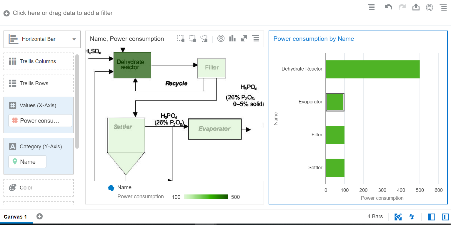
Once in the visualize tab, the user can bring in the NAME column into a canvas and should see map viz render with the acid process image as map background with the custom map layer generated in the previous step on top of it.

We can bring in a power consumption metric to the color edge to show how much power is consumed in various stages.

Also other business charts can be brought into the canvas and the normal DV interactions such as brushing and filtering can be used with image background.

   Another example of image background with polygon layer is that of a picture of motor bike shown     below

An example of image background with point layers is shown below

This is a very powerful feature and can be treated like a custom visualization for different images.
Thanks for reading our blog !

How Regex can enhance Data Preparation?

Is simple find-and-replace not sufficient for your need in Oracle Analytics Data Preparation ? Regular Expression Replace functionality is bringing great new powerful abilities with pattern matching in Oracle Analytics Data Prepare. We will see what it has got to offer, in this blog.
First, take a quick look at the video which explains briefly about this feature.

Oracle Analytics now allows users to utilize the full potential of Regular Expressions aka Regex in pattern matching of column text in OAC Data Preparation or Data Set editor. Before we jump into the feature, let's recollect the basics of regular expressions. You can skip this part if you’re already familiar with Regular Expressions.

Regular Expressions in a nutshell

Regular Expressions is a powerful tool for matching patterns. A pattern can be a word or a specific character or sequence of characters, occurring once or multiple times. Regex can also help you find words occurring in a specific format, like email address. We will only address some of the useful Regex patterns in this blog entry, which will still help you kick-start Regex Replace in OAC Data Preparation.

For starters, let's see some of the commonly used Regex patterns :

Let's start with a pattern to match one or more digits. ‘\d+’ can be used to find the digits from 0-9 anywhere in the string. The backslash ‘\’ is used as escape character, ‘d’ is the shorthand code for digits and ‘+’ sign denotes one or more occurrence. Other useful patterns are:

• w            Any alphanumeric character
• W           Any non-alphanumeric character
• d             Any digit
• D            Any non-digit character
• .              Any character
• *             Zero or more repetitions
• +             One or more repetitions
• ?             Optional character

Character Classes or Character Sets

When you want to match only one out of several characters, Character classes or Character-sets can be used. For eg. to match an a or e, we can use [ae]. The pattern ‘gr[ae]y’ matches gray and grey but not Grey or graay.

It is also possible to specify a range with [] brackets. For eg. [0-9] matches a digit from 0-9, [a-z] matches a letter from a to z. Multiple character ranges can also be used. For Eg. [A-Z0-9] matches an uppercase alphabet followed by a digit. Remember, the patterns are case-sensitive!

Grouping Patterns

In Regex, group of characters can be defined for capturing and processing the data. Let's do this with an example. Consider the text ‘ABSD0028’ which has two parts – alphabets(ABSD) and digits(0028). If we have to write a pattern to split the text into two parts, we can do so by grouping the characters with parenthesis and each group can be captured using back-references. Here is our pattern.

([A-Z]+)(\d+)

Back-references

Now, having learnt about the grouping, we must know how useful are they in the real-world scenario. The main purpose of grouping in regular expressions is to use one or more groups in the output. Let’s consider the above example. We grouped the text into two parts. We can refer these parts using back-references and construct a new text. Naming of the back-reference parameters might vary depending upon the platform/programming language on which Regex engine works. In OAC, back-reference parameters are denoted by a ‘$’ sign followed by the order of occurrence of the group.  For eg. in the pattern ([A-Z]+)(\d+), ‘([A-Z]+)’ will be referred as $1 and ‘(\d+)’ will be referred as $2.

Alternation

Alternation is the ‘OR’ operator in regular expression. To match red or green or blue, use red|green|blue. To match ‘red color’ or ‘blue color’ use grouping, for eg. (red|blue) color.

Constructing a pattern

Now, let’s construct a pattern which we could use in Regex Replace. Consider extracting email handle from an email address. Email ids are in the following format: <some_text>@<org_name>.<com>. Let’s split this format into three parts – first part, the email handle, second part, the ‘@’ symbol and third part, the domain. The first part could include alphanumeric characters with special characters like ‘_’ and ‘.’. So, the pattern for this part would be: ‘[A-z0-9_\.]+’. We can use the second part as it is. And, the third part is going to be alphabets with ‘.’, the pattern would be ‘[a-z\.]+’. Now, if we combine the three parts, we get the following pattern:

([A-z0-9_\.]+)@([a-z\.]+)

So, what’s new with Replace in OAC Data Preparation?

Let’s see what’s new in Replace functionality. For the demo purpose, I have created a project with a data set called Customer Profile, which has customer details like JOB_LEVEL, Email address, Phone number, Occupation, Education etc.

Earlier, in Data Preparation, there was just plain search and replace feature in the context menu of the columns. There was no option to specify a partial or entire match. Now, there are three options available in Replace page as radio buttons.

       a.   Match partial values
       b.   Match entire values only
       c.   Use regular expression

When option a is selected, matches are found in both partial and entire values of the text. Let’s see how ‘Match partial values’ work in the column Occupation. In the Prepare tab of the project, right-click on the column Occupation and select Replace.

You can see the following values in Occupation: 

Enter ‘Manual’ in String to replace and ‘Worker’ in New String. Select ‘Match partial values’. You will notice that both ‘Manual’ and ‘Skilled Manual’ are modified to ‘Worker’ and ‘Skilled Worker’ respectively.

Now, select ‘Match entire values only’ with same input. You will notice that only ‘Manual’ is modified to ‘Worker’ and ‘Skilled Manual’ remains the same. This option comes in handy when the requirement is specific to replace the entire values alone.

We will explore option c, ‘Use regular expression’ with rest of the examples.

Use of Alternation or ‘|’

In the column ‘ENGLISH_EDUCATION’ let’s remove the words ‘Partial’ and ‘Degree’ from the values.

Enter ‘Partial|Degree’ in String to replace, leave New String as blank and select ‘Use regular expression’. Now you will see that ‘Partial’ and ‘Degree’ are removed from the values like ‘Partial High School’, ‘Partial College’ and ‘Graduate Degree’ correspondingly.

You can use the ‘|’ symbol as the ‘OR’ operator to include more than one value to match. As you might have noticed, this eliminates multiple steps when more than one matches need to be replaced with a single value.

Obfuscation, using literal matches

Obfuscation is a significant step in Data Preparation, as it improves the privacy and security of sensitive content. Popular candidates for obfuscation could be Social security numbers, phone numbers, account numbers etc. With powerful features of regular expressions, it becomes easy to obfuscate in OAC. Let’s see how to do that with an example. In our data set, let's obfuscate the column Phone. If you notice the values of this column, it is divided into three parts. The first three digits within parenthesis, next three digits separated with a dot (.) from the last four.

Let’s replace the digits with ‘x’ mark. Enter ‘\d+’ in String to replace and enter ‘xxx’ in New String (‘[0-9]+’ and ‘\d+’ can be used interchangeably). Select Use regular expression and you will see all the numbers are replaced with ‘xxx’. Various patterns can be used according to the requirement.

Extraction with Back-reference

Let’s see how to extract specific part of the text using regular expression. Consider the column Email_address from our data set. Let’s extract the email handle from the email address.

As you might recall the pattern we constructed in the Regex example for the email address – ([A-z0-9_\.]+)@([a-z\.]+) can be divided into three parts. We’re interested in the first part, which is the email handle. Enter the pattern ‘([A-z0-9_\.]+)@([a-z\.]+)’ in String to replace and enter $1 in the New String and select Use regular expression. Now, you will just see the first part of the email address in the column. You may rename the column name as email_handle.

So, once we group and divide a text according to our need, we can use them in the output as back-references. This might be helpful where the data has multiple columns combined into one. For eg. IL-Chicago, where State and City combined into one column. Columns with log entries, timestamps etc could be interesting candidates for extraction using back-references.

Enriching data with Regular Expressions

When we want to enrich the existing data in a highly customized format, we can use grouping and back-references together to make a powerful combination to transform data in one shot. Let’s enrich the column JOB_LEVEL by inserting some text in between.

Similar to the example we saw in Grouping Patterns, JOB_LEVEL has two parts – alphabets first and digits next. The pattern ‘([A-Z]+)([0-9]+)’ can be used to match and split into two parts. Let's insert the text ‘_000’ between two parts. Enter ‘([A-Z]+)([0-9]+)’ in String to replace, ‘$1_000$2’ in New String and select Use regular expression. You will see the JOB_LEVEL is transformed into an enriched column. This could be helpful when the data is expected to be in a specific format.

What we have seen here in this blog is, just the tip of the ice-berg. A lot more can be done with Regular Expression Replace and it can be a powerful combination in OAC Data Preparation.

Thanks for reading this blog!

How to retrieve valuable information related to your ML models in Oracle Database - Part II

In part I of the blog on this topic (http://oracledataviz.blogspot.com/2020/04/how-to-retrieve-valuable-information.html), we talked about the various data mining views that store information about every ML model that gets created in the Oracle database. These views have information about ML models size, models settings, attributes used in the models etc. This information is available for each ML model created in the database irrespective of the mining function or the algorithm used.

We also talked about one particular view called ALL_MINING_MODEL_ViEWS which contains the names of all the underlying model views that gets created behind the scenes every time we create an ML model. The number and kind of views that get created differ from one algorithm to another. An ML model built using Naive Bayes algorithm will have a set of related model views. An ML model built using Decision Tree will have another set of related model views created and so on.

In this blog, let’s look at these specific model Views that get created for different algorithms.

Let us consider the same Sample Problem discussed in Part I of the blog which is to determine a customer’s response to an affinity card program. Let’s build an ML model called DT_TEST using Decision Tree algorithm. (Refer to Part I for Model training syntax details).

Once the model is created, if you query ALL_MINING_MODEL_ViEWS for the model_name as DT_TEST, you will find that the following underlying views have been created.

These view names have a fixed format. It begins with DM$V followed by an alphabet that is specific to the model view followed by the model name. DM$V<Alphabet><Model Name>. 

Let’s look at some of these views, see what information they contain and how to visualize them using Oracle Analytics.

a) DM$VCDT_TEST – This is the scoring cost view and describes the scoring matrix for classification models. The view has actual_target_value, predicted_target_value and cost.
Conclusion
x

     b) DM$VGDT_TEST - This view describes global statistics related to the model build like number of rows used in the model build, convergence status and so on.

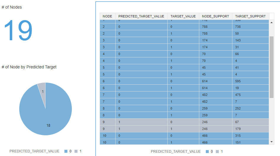
     c)  DM$VIDT_TEST - This is the node statistics view and describes the statistics associated with individual nodes in the decision tree. The statistics include a target histogram for the data in the node. For every node in the tree, this view has information about predicted_target_value,  actual_target_value and node support.

Here's a sample visualization of this information for the DT_TEST model that resulted in a tree with 19 nodes.

     d) DM$VMDT_TEST - This view describes the cost matrix used by the decision tree build.

     e) DM$VODT_TEST - This view contains the high level node description. It contains the Node and Parent information that allows us to understand the hierarchy of nodes. For every node, there is information about the attribute associated with the node, operator (IN, > , <> etc) and the attribute value. The attribute value is stored as an XMLTYPE in the view. In order to visualize it within Oracle Analytics, extract the string value from the XML in the data set creation similar to what's shown below.

Once the data set is available in Oracle Analytics, a tree diagram helps in understanding the hierarchy of nodes in the decision tree. Attribute details about each node is also available in this view providing more insight about attributes that are relevant in the input dataset.

     f) DM$VPDT_TEST - This is the split information view and describes the decision tree hierarchy and the split information for each level in the Decision Tree. For each node in the tree, this view has details about the attribute associated with the node and the split type (Main/Surrogate).

     g) DM$VSDT_TEST - This is the computed settings view and lists all the algorithm computed settings as a name-value pair.

     h) DM$VTDT_TEST - This is the target map view and describes the target distribution. The view contains target_value, target_count and target_weight information.

     i) DM$VWDT_TEST - This is the alert view and lists all the alerts issued during the model building process.

While a Decision Tree model results in a specific set of views , a Naive Bayes model called NB_TEST will result in a slightly different set of views as shown below.

Conclusion

Oracle Database maintains a lot of valuable information in several dictionary views when a mining model is built. The information in these views helps in understanding several aspects like what attributes are important in the input data set, what is the distribution of the target value, details about the model that can help in iterative-ly improving the overall accuracy of the model predictions and so on. Oracle Analytics helps in visualizing all this information in an intuitive and interactive manner.

Using of Session and Repository variables in Oracle Analytics (OAC and OAS)

In this blog, let's explore the different types of variables existing within OAC 5.6 infrastructure with a specific focus on repository variables and session variables. We will be looking at how we can leverage these two types of variables in Oracle Self Service Analtyics.

Repository Variables:

A repository variable has a single value at any point in time. Repository variables are substitutes for literals and constants and the Oracle OAC server substitutes this value in any logical expression, either in the semantic layer metadata or in a project/analysis calculation or filter expression. There are 2 different types of repository variables :

1) Static Repository variable

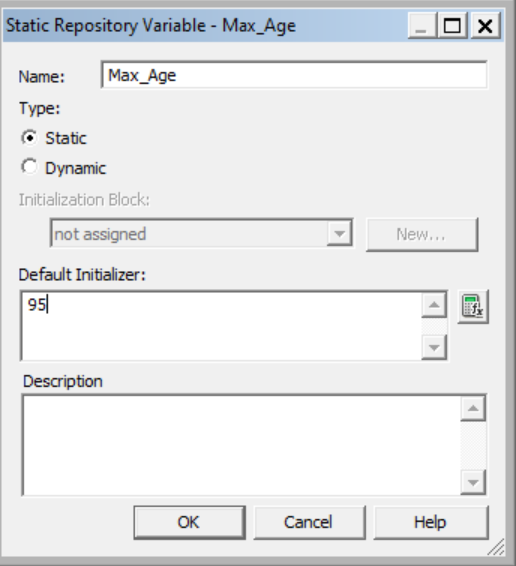
The value of a static repository variable is initialized inside the variable dialog interface of OAC Admintool. The value then persists and does not change until an administrator decides to change it.
For example, you can define a static variable called Max_Age and assign a value to it.

The syntax to access a static repository variable from any logical calculation or filter is as follows :
VALUEOF("<name_of_static_variable>"). In the case of the example it will be something like :

2) Dynamic Repository Variable

Dynamic repository variables in the same way as static variables, but the values are refreshed by data returned from pre-defined queries in the semantic layer (Repository) metadata. When defining a dynamic repository variable, one first creates an 'initialization block' that contains a specific SQL query. You also set up a schedule that the Oracle BI Server will follow to execute the query and periodically refresh the value of the variable.
For example, assume you have a table that contains information on various trips done by a cab service.

Now you have to keep track of the trip which has the traveled the longest distance.
Distance is a metric that will be calculated using some spatial functions on the columns TRIP_START and TRIP_END.
Let us say that there are a few thousand records in your data, and so far the maximum distance is, say 1000 miles. Without using dynamic repository variables, you would describe the trip containing the longest distance with an expression such as: Trips.distance >= 1000

This content statement becomes invalid as new data is added to the recent source which might actually change the value of the maximum distance. Instead of modifying the variable definition manually, dynamic repository variables can be set up to do it automatically.

To create dynamic repository variables, you create both the dynamic variables and an initialization block, then match both together.

To create an initialization block, go to Action->New->Repository->Initialization block.

Give it a name and schedule the time & refresh interval. Then click on the Edit Data Source and point it to the correct connection pool. Type in the sql after choosing the correct connection pool.

In our example : 

select trip_id, sdo_geom.sdo_distance(trip_start, trip_end, 0.005) distance

from trips

where  sdo_geom.sdo_distance(trip_start, trip_end, 0.005)=

(select max(sdo_geom.sdo_distance(trip_start, trip_end, 0.005)) from trips)

The first column returned by the above sql is the trip_id and the second column is the max distance. In our example, let's assign these values to two distinct dynamic repository variables :

Click on Edit Data Target and add two variables and name it Longest Trip and Maximum_Distance to associate with the query result.

Simply save the RPD, upload it on to an OAC instance and bring the subject area into a project or Analysis. The syntax for accessing the dynamic repository variables is the same as for a static repository variables.

VALUEOF("<name_of_dynamic_repo_variable>")

Create 2 custom calculations for the 2 dynamic repo variables with the following syntax:
VALUEOF("Longest Trip")
VALUEOF("Maximum_Distance")
and display it on a DV canvas.

A common use of these variables is to set filters for use in Oracle Analytics.

Session variables :

Session variables are similar to dynamic repository variables in that they obtain their values from initialization blocks. Unlike dynamic repository variables, however, the initialization of session variables is not scheduled. When a user logs-in and begins a session, the Oracle Analytics server creates new instances of session variables and initializes them.
Unlike a repository variable, there are as many instances of a session variable as there are active sessions (users) on the Oracle BI Server. Each instance of a session variable could be initialized to a different value. Here again, there are 2 types of Session variables :

1) System Session Variables:

System session variables are session variables that the Oracle Analytics server use for specific purposes. They have reserved names and cannot be used for other kinds of variables. There exists many system session variables, some of them are listed below :

USER	This variable holds the value the user enters with login name. This variable is typically populated from the LDAP profile of the user.
USERGUID	This variable contains the Global Unique Identifier (GUID) of the user and it is populated from the LDAP profile of the user.
GROUP	It contains the groups to which the user belongs. When a user belongs to multiple groups, group names are concatenated separated by semicolons (Example - GroupA;GroupB;GroupC).
ROLES	This variable contains the application roles to which the user belongs. When a user belongs to multiple roles,  the role names are concatenated separated by semicolons (Example - RoleA;RoleB;RoleC).
ROLEGUIDS	It contains the GUIDs for the application roles to which the user belongs. GUIDs for application roles are the same as the application role names.

Let us consider the system session variable USER which holds the value the user enters as his or her logon name. The syntax for accessing the System session variable in DV is as follow.

VALUEOF("NQ_SESSION.<name_of_system_session_variable>")

This is similar to syntax for repository variables but with prefacing their names with NQ_SESSION.

This syntax can be used as an argument for in any logical calculations, or custom filters. When dragging the custom calculation on to a DV canvas, the value of system session variable is seen.

The Oracle Analytics documentation will help you get an exhaustive list on all the system session variables along with their description. 

2) Non-System Session Variables:

These are system variables that an administrator can create using the Oracle BI Administration tool. They are part of the semantic layer of Oracle Analytics. The use of Session variable is wide, they are basically holding session based value that refresh everytime a user connects, using any particular predefined SQL. An example of non-system session variables could be to set user filters for example.

To define Non-System Session Variables, simply go to the variable manager in the admin tool and click on Action -> New -> Session -> Initialization block and replicate the one shown in the below diagram.

Now a non system session variable called Currency is created and the user can now access them in DV using the same syntax of system session variables. VALUEOF("NQ_SESSION.<name_of_non-system_session_variable>")

Drag and drop this calculation on a canvas to see the value of the currency variable set.

How to retrieve valuable information related to your ML models in Oracle Database - Part I

Oracle Database offers powerful Machine Learning algorithms that enable data analysts to discover hidden patterns and insights. With Oracle Machine Learning (OML), you can build and apply predictive models inside the database that help predict customer behavior, identify cross-selling opportunities, build customer profiles and detect anomalies. These algorithms are implemented as SQL functions that can be directly invoked inside the database without moving the data and thereby leveraging the inherent strengths of the database.

OML offers a broad range of in-database algorithms to solve different kinds of business problems. For classification type of problem, there are algorithms like Naïve Bayes, Decision Tree, Support Vector Machine etc. For clustering , there is Enhanced K Means, O Clusters and so on.

For every ML model that is created in the database, different kinds of information related to the model are stored in several specific DB Tables and Views within the database.

In this blog, let’s create a simple OML model and explore the various mining model views that are created with the model in the database and how these can be leveraged to get valuable information about the model itself.

Sample Problem 

Let’s assume we are given a demographic data set about a set of customers and we would like to predict the customer response to an affinity card program using classification function based on Decision Tree algorithm. This dataset contains 3000 records with customer attributes like cust_gender, cust_marital_status, education, occupation, household_size and so on. Grain of this dataset is cust_id so every record has a unique cust_id.

Create an ML Model

Let’s create a classification model using Decision Tree (DT) to address this problem. The database offers several options to enhance the overall accuracy of a model like how to handle missing value for predictors, outlier treatment for predictors, method for binning high cardinality data and so on. For the purpose of this blog,  let us use the basic minimum steps to build a DT model.

Default mining algorithm used to build a classification model is Naïve Bayes. In order to build a Decision Tree classification model, we need to first create and populate a settings table and use this settings table as input to the model building procedure.

- Sample Syntax to create/populate model settings table

CREATE TABLE dt_sh_sample_settings

(setting_name  VARCHAR2(30),

setting_value VARCHAR2(4000));

                  INSERT INTO dt_sh_sample_settings VALUES

    (dbms_data_mining.algo_name, dbms_data_mining.algo_decision_tree);

- Sample Syntax to create a Classification model using Decision Tree algorithm.

                BEGIN

                DBMS_DATA_MINING.CREATE_MODEL(

model_name          => 'DT_TEST,

mining_function     => dbms_data_mining.classification,

data_table_name     => 'mining_data_build_v',

case_id_column_name => 'cust_id',

target_column_name  => 'affinity_card',

settings_table_name => 'dt_sh_sample_settings');

END;

Query model related information

Every time an ML model is built, there are several details about the model that are stored in a few data mining related views. Following section describes the important mining views in the database that can be leveraged to understand the model details. The information from these views can be easily visualized using Oracle Analytics Cloud.

a)       ALL_MINING_MODELS – This view in the database describes all the mining models accessible to the current user. It has details about the model owner, model_name, mining_function used in the model (Classification, Regression, Clustering and so on) , algorithm used to build the model (Naïve Bayes, Decision Tree and so on) , model creation date , model size and so on.  This view has one record for every OML model created.
There are two related views: 
             i) DBA_MINING_MODELS that describes all the mining models in the database.
             ii) USER_MINING_MODELS  that describes the models owned by the current user.

Information in this view can be visualized within Oracle Analytics Cloud by creating a dataset sourcing from this view.

Important Note: When you navigate to the schema in the data set creation screen, these data mining views are not listed as objects. However, you can enter a custom SQL similar to ‘Select * from ALL_MINING_MODELS’ to retrieve the model details.

Here's an example of the output of the ALL_MINING_MODELS view related to the model called DT_TEST.

b)       ALL_MINING_MODEL_ATTRIBUTES – This is an important view and contains information about the columns in the training data that were used to build the model. For each attribute, details about the attribute name, datatype, whether attribute is Target etc is available in this view. When this model is applied on a data set for scoring, columns with the same names and data types should be available in the scoring data set. In this case as well, there are two related views DBA_MINING_MODEL_ATTRIBUTES and USER_MINING_MODEL_ATTRIBUTES. 

Here's a sample output of this view for a model called DT_TEST as visualized within OAC. 

c)     ALL_MINING_MODEL_SETTINGS – This view describes the settings of the mining model. Here's a example of the model settings for a model called DT_TEST visualized using OAC.

d)       ALL_MINING_MODEL_VIEWS - This is another important view that provides slightly different kind of information. Every time an ML model is created in the database, there are several underlying model views that get created relevant to this model. The number and kind of these model views created differ from algorithm to another. An ML model built using Naive Bayes algorithm will have a set of related model views. An ML model built using Decision Tree will have another set of related model views created and so on. For example, consider a Decision Tree model called DT_TEST. Following are the model views created :              

Note that the view names have a fixed format. It begins with DM$V followed by an alphabet that is specific to the model view followed by the model name. DM$V<Alphabet><Model Name>. 

We will refer to the details on these specific model views for various mining algorithms in an upcoming Part II of blog entry on this topic. 

Conclusion

For every ML model that is created in the Oracle Database, there are a lot of metadata about the model available as part of the dictionary views. If you are interested in knowing more about this topic, kindly refer to Oracle Documentation, or stay tuned for the second part of this blog entry coming soon.