Custom Scripts in Oracle Analytics Desktop - Geocoding

Oracle Analytics is a comprehensive unified platform offering services including self-service visualizations, powerful data-prep tool, advanced analytics and augmented analytics.

In this blog, we are going to explain the use of leveraging custom-scripts using Oracle Analytics Desktop (OAD) and few tips and tricks to install additional custom Python packages that do not come by default with the Python engine.

Let us take the following scenario : a user has a dataset with an address column and needs to plot these address on a map visualization. In technical terms, he needs a geo-coding capability which converts valid addresses to corresponding Lat & Longs which can then be used for plotting on a map. .

One way for the user to achieve that would be to leverage Spatial Studio application (free with Oracle Database). Spatial Studio is a self-service web application that makes it easy for users to create interactive maps and perform spatial analysis on their business data. User just needs to upload his dataset into Spatial Studio and the geocoding service can then be invoked to find the corresponding Lat/Longs. Once done, the user can simply visualize his dataset in Oracle Analytics platform. 

But the user has another option to achieve the same result : using Custom Scripts in OAD.

Oracle Analytics Desktop comes with in an in-built Python engine. This Python engine is wrapped around an internal layer called DVML which needs to be installed for a user to run custom scripts on OAD.

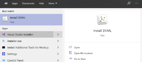
Search for Install DVML and install the application

As of OAD 5.6, DVML uses Python version 3.5.2. OAD expects a particular format for a script to be accepted and executed by it's Python engine. This should be an .xml file with well-defined inputs, outputs and options tags. We can break down the process of creating a custom Python script on OAD into 2 simple steps

1. Have the script working on a standalone Python editor
2. After completing the first step, wrap the script in the form of an XML wrapper by properly defining the input and output tags and also by making sure that the resultant dataframe of the Python script matches with the output structure defined in the XML.

Coming back to our scenario where a user wants to perform geocoding, this functionality can easily achieved in Python through a package called geopy. 

A custom python script can simply call the geocode function from this package, using the Address column as argument. If user creates such a custom Python script and uploads it into OAD, he can then simply invoke it from an Oracle Analytics Data Flow by using the "Apply Custom Script" node. This will let the OAD's Python engine to execute the geocoding script. But at this point, when the dataflow is executed the user is likely to see an error...

Checking the logs it becomes clear that geopy package was not found by DVML python engine. This is an indication that the geopy package needs to be installed as a part of DVML. When a user installs DVML, it comes with default set of commonly used Python packages like pandas, numpy, scikit-learn, etc. But how to install new python packages into DVML ?

Installing Python packages into DVML

Here are the steps to be followed to install Python packages into DVML on a MS Windows machine :  search for DVML Runtime and choose the option "Open File Location".

This will open the folder which has the shortcut to DVML. To get the actual location as to where the DVML files are installed, right click on the short-cut and choose the options "Open File Location".

If the default path was chosen during the initial DVML installation (MS Windows machine), the DVML files will be under this directory : C:\Program Files\DVMLRuntime\PCbuild\amd64

Open cmd prompt and run it as an administrator. Navigate to the above path and type in the following command : python -m pip install geopy

This should install the geopy package as part of DVML. 

If you encounter any issues in the above step you can try this alternative approach : search for DVML Runtime and open it as an administrator. This open up a Python prompt where a user can type in python commands. Type the following commands to install python packages.

from pip._internal import main

main.main(["install","geopy"])

In both approaches, replace geopy with the package you want to install and it should install the package into DVML. Once the user has imported all the relevant packages, these packages can be imported and used in the OAD custom scripts. Restarting the OAD and running the geocoding dataflow should now result in a successful execution.

In this approach of geocoding, the user needs not switch between applications or do multiple upload or download of files to get the resultant output. The user can stay in OAD, run the Python script and get the resultant output.

Anything that you can do in standalone Python editor like a Jupyter notebook is possible in OAD by using Dataflows and custom scripts.

As of today, custom scripts import are only applicable to desktop or On Prem (OAS) versions of Oracle Analytics. The cloud version OAC is being worked on to support similar capability in the near future.

Geocoding Script Details

As evident from the above pic, geopy package was imported into the script along with few other packages. There are many providers who offer the geocoding capability. Some of them include Google, OpenStreetMap, Bing, etc. In order to use Google or Bing service, the user should sign up on their platform and get a valid API key to pass it along the geocode request. OpenStreetMap offers geocoding service called Nominatim which offers free geocoding service without the need for the API key. However it requires a user_agent to be passed. This can be the App id of the application or just an email address.

In this script, I have used the Nominatim geocoding service and have used my email address as the user agent. Also another aspect about the Nominatim geocoding service is that there a limit on the number of requests it can serve at a moment. Hence I have used the ratelimiter package to send only one row per second to the Nominatim server. A place name will be passed to the Nominatim geocoding service which results in the address and the Lat/Long coordinates of the place. The results are then passed into the output dataframe.   

Thanks for reading the blog and you can download the geocoding custom script here for your future references.

Parameters of Random-Forest Algorithm for Classifications

Oracle Analytics includes several Machine Learning algorithms that enable data analysts to identify patterns in their data and make predictions on it. These various algorithms support different type of models : classifications, clustering or numeric predictions. Each algorithm offers several hyper-parameters to control the model training process and that can be manually tuned to improve overall model accuracy. It is important to understand these hyper-parameters to tune your training process in order to quickly get to the most accurate predictive model.

If we look in particular at classification models -both binary and multi-classification, Oracle Analytics offers several algorithms to perform it : 

                                     

Each of these come with a set of hyper-parameters that can be configured. In this blog, let us understand in detail on the Random Forest algorithm and review these parameters, they are actually fairly simple to understand and leverage :

Random Forest for model training

Random Forest is a classification algorithm that builds several Decision Tree models on the data and predicts using all these trees, called 'a forest of trees'.This algorithm builds each individual decision tree is by choosing a random sample data from the data set as the input. At each node of a tree, only a random sample of predictors is chosen for computing the split point. This introduces variation in the data used by the different trees in the forest.

Following is the list of hyperparameters available for this algorithm (for both binary classifications and multi-classifications): 

    

Let us understand these parameters in detail: 

• Target: This is the column with actual values which we wish to learn the model on. In case of binary classifications, the target must have two possible values (Yes/No, 0/1 and so on). In case of multi classifications, it can have more than two outcomes ( Low/Medium/High, North/East/South/West and so on).

• Positive class in Target: This allows the user to specify a value of the Target column that is interpreted as a positive class in the target. In order to classify the possible output values, the algorithm needs Positive and Negative classes. ‘Yes’ is the default option.

• Number of Trees in the forest: This hyper-parameter is considered to build the ensemble or forest of the model. It accepts a number between 2 and 100, with a default value of 10. A general guidance is, the more trees in the forest, the better the results. A higher number of trees means means more samples created from the initial training data-set. That reduces the biased-ness in the data used for training and can achieve more realistic results. However, increasing number of trees value will have performance implications for large datasets. 10 is the default value.

• Sample Size for a Tree: this determines the size of the sample data that is used for any single tree to predict the outcome. You can control the degree of randomness with the sample size parameter as increasing the sample size results in less 'variation' (randomness) in data for the individual trees in the forest. The best sample size is actually equal in size to the size of the original dataset : some rows are not selected while others are selected more than once. This typically provides near-optimal performance. However, in real-world applications, you may find that adjusting the sample size iteratively can lead to improved performance. This accepts a number between 500 and 10,000 with 500 as the default value.

• Number of Features for a Tree: This accepts a number between 2 and 10. Increasing the number of features generally improves the performance of the model as there are higher number of options to be considered at each node. However, this can decrease the diversity of an individual tree which is the significant aspect of random forest. Also, by increasing the features, the speed of algorithm decreases. Hence, we must find the right balance and choose the optimal value. 3 is the default value.

• Minimum Node Size: This is the minimum size of each leaf nodes in the decision tree and accepts any value between 10 and 100. This will constrain the tree into not being able to have a terminal node with less records than this number. When the limit is set high, it causes decision trees to be smaller and hence take less time to compute the samples. Setting it low leads to trees with a larger depth which means that more splits are performed until the terminal nodes, which can provide deeper insights on the data. Lower values are believed to generally provide good results, but performance can potentially be improved by tuning it. 50 is the default value.

• Maximum Depth: This represents the depth of each tree in the ensemble or the forest. The depth is the number of levels in the tree 'splits' hierarchy : how many levels from the first split to the furthest leaf level. The deeper the tree, the more the tree captures variance information about the data. The objective should be to expand each tree until every leaf is as pure as possible. A pure leaf is one where all the data comes from exactly the same class.  This parameter combines wiht Node Size as well, and has a direct impact on training performance : more levels require more processing time to train a model. Maximum Depth can be set up to 10 with 5 being the default.

• Maximum Confidence: This represents the confidence interval the model can take and can be used to rank the rules and hence the predictions. It is a measure of how sure the model is that the true value lies within a confidence interval computed by the model. This determines the likelihood of the predicted outcome, given that the rule has been satisfied. For example, consider a list of 1000 patients. Out of all the patients, 100 satisfy a given rule say, high fasting blood sugar level. Of these 100, 75 are likely to have heart disease, and 25 are not likely to have. The confidence of the prediction (likely to have) for the cases that satisfy the rule is 75/100 (75%). Maximum confidence parameter accepts a value between 1 and 100 with 80 being the default.

• Train Partition Percent: This is used to specify the percentage of training data that should be used to build model and the remaining will be used for internal testing purpose of the model. During the model creation process, the input data set is split into two parts to train and test the model based on the Train Partition Percent parameter. The model uses the test portion of the data set to test the accuracy of the model that is built. Default value is 80 which means 80% of the data is used to train the model and 20% to test model accuracy.

• Balancing method: This is used when there is an imbalance classification of the given samples : a skewed number of records have a given value (vast majority of 'No' and very few 'Yes').... In such situations, a method is applied in the algorithm to re-balance the set for better training : Under Sample, Over Sample and None are the options available. When the dataset is imbalanced, with majority of the records having a target attribute value of ‘No’, with under-sampling, the set of records where the target attribute is ‘No’ will be under-sampled to provide the same number of records as those with a value of ‘Yes’. When the dataset is small, an oversampling method can be used, and its effect is the opposite of under-sampling. Over-sampling will look at records having a target value of ‘Yes’ and over-sample these until it has the same number of records as those of the other target values. Default is Under Sample.

Case Study

To explore more about Random Forest algorithm and the effect of its parameters, let us consider a customer demographic data set with 1500 records. This dataset contains customer attributes like cust_gender, cust_marital_status, education, occupation, household_size and so on and we would like to train a model that will predict the customer response to an affinity card program with two possible outcomes Yes/No.

Here’s the sample dataset:

 

First, upload this dataset in Oracle Analytics. Next, create a dataflow with this input dataset and choose Train Binary Classifier step. Choose Random Forest for Model Training as the script.

A list of hyperparameters to train the model with default values as described in the previous section is displayed. Let us understand the effect of these hyperparameters on the model quality in different iterations.

Iteration 1: Let us leave these hyperparameters with default values and execute the dataflow. Successful dataflow execution creates a Machine Model which can be viewed from the Machine Learning tab. Let us right click on the model and inspect it to know more about its quality. With default parameter values, following is the model’s quality. 

Model accuracy is 76% which is computed as (True Positive + True Negative)/Total = (65+163)/300

Precision is 54% which is computed as (True Positive)/(True Positive+False Positive) = 65/(65+55)

False Positive Rate is 25% which is computed as False Positive/Actual Number of Negatives = 55/218

Iteration 2 : Let us increase the Sample Size of the tree from default 300 to 1500( as we have 1500 records in our input dataset). Let’s rebuild the model by executing the dataflow. Upon inspecting the model quality, we notice that while accuracy remains at 76%, precision has improved from 54% to 55%.

Iteration 3: Let us increase the number of trees from default 10 to 30 and Maximum depth from default 5 to 7.  Rebuild the model and inspect model details. 

We notice that the model accuracy has improved to 77%, precision has improved to 56% and False Positive Rate has dropped from 25% to 24%.

Conclusion:

Every Machine Learning algorithm in Oracle Analytics comes with a set of model training hyperparameters that can be tuned to improve overall accuracy of the model created. Given that the model building process via Dataflows is a fairly simple and intuitive process, it becomes easy to iteratively change the model hyperparameter values, inspect the model quality and subsequently arrive at a model of desired accuracy in a reasonable amount of time.