Friday, November 24, 2017

Measure effectiveness of your Marketing Campaign using Oracle DV ML

In this blog we will talk about Cumulative Gains chart and Lift chart created in Oracle Data Visualization for Binary Classification ML models and how these charts are useful evaluating performance of classification model.

What are Cumulative Gain &Lift charts and what are they used for?
Let us suppose that a company wants to perform a direct marketing campaign to get a response (like a subscription , purchase etc) from users. It wants to run marketing campaign for around 10000 users out of which only 1000 users are expected to respond. But the company doesn't have a budget to reach out to all the 10000 customers. To minimize the cost company wants to reach out to as less customers as possible but at the same time reach out to most (user defined) of the customers who are likely to respond. Company can create ML models to predict which users are likely to respond and with what probability. Then the question comes which model should I choose? Which ML model is likely to give me the most of number of respondents with as less selection of original respondents as possible? Cumulative Gains and Lift chart answers these questions.

Cumulative Gains and Lift chart are a measure of effectiveness of a binary classification predictive model calculated as the ratio between the results obtained with and without the predictive model. They are visual aids for measuring model performance and contain a lift curve and baseline. Effectiveness of a model is measured by the area between the lift curve and baseline: Greater the area between lift curve and baseline better the model. One academic reference on how to construct these charts can be found here. Gains & Lift charts are popular techniques in direct marketing.

Sample Project for Cumulative Gains and Lift chart computation
Oracle Analytics Store has an example project for this that was build using Marketing Campaign data of a bank. This is how the charts look like:


Scenario: This Marketing Campaign aims to identify users who are likely to subscribe to one of their financial services. They are planning to run this campaign for close to 50,000 individuals out of which only close to 5000 people i.e., ~10% are likely to subscribe for the service. Marketing Campaign data is split into Training and Testing data. Using training data we created Binary classification ML model using Naive Bayes to identify the likely subscribers along with prediction confidence (note that the Actual values i.e., whether a customer actually subscribed or not is also available in the dataset). Now they want to find out how good the model is in identifying most number of likely subscribers by selecting relatively small number of campaign base(i.e., 50,000).

ML models are applied on Test data and got the Predicted Value and Prediction Confidence for each prediction. This prediction data and Actual outcome data is used in a dataflow to compute cumulative gain and lift values.


How to interpret these charts and how to measure effectiveness of a Model:
Cumulative Gains chart depicts cumulative of percentage of Actual subscribers (Cumulative Actuals) on Y-Axis and Total population(50,000) on X-Axis in comparison with random prediction (Gains Chart Baseline) and Ideal prediction (Gains Chart Ideal Model Line) which depicts all the 5000 likely subscribers are identified by selecting first 5000 customers sorted based on PredictionConfidence for Yes. What the cumulative Actuals chart says is that by the time we covered 40% of the population we already identified 80% of the subscribers and by reaching close to 70% of the population we have 90% of the subscribers. If we are to compare one model with another using cumulative gains chart model with greater area between Cumulative Actuals line and Baseline is more effective in identifying larger portion of subscribers by selecting relatively smaller portion of total population.

Lift Chart depicts how much more likely we are to receive respondents than if we contact a random sample of customers. For example, by contacting only 10% of customers based on the predictive models we will reach 3.20 times as many respondents as if we use no model.

Max Gain shows at which point the difference between cumulative gains and baseline is maximum. For Naive Bayes model this occurs when population percentage is 41% and maximum gain is 83.88%

How to compare two models using Cumulative Gain and Lift Chart in Oracle DV:
To compare how well two ML models have performed we can use Lift Calculation dataflow(included in the .dva project) as a template and plug in output of Apply Model dataflow as data source/input to the flow. Add the output dataset of Lift Calculation to the same project and add columns to the same charts as shown above to compare. Please note that the data flow expects dataset to contain these columns(ID, ActualValue, PredictedValue, PredictionConfidence). This is how it will look like when we compare two models using same visualizations:

 
.
Are you an Oracle Analytics customer or user?

We want to hear your story!

Please voice your experience and provide feedback with a quick product review for Oracle Analytics Cloud!
 

Wednesday, November 22, 2017

Which ML model is the right one for me?

In the world of Machine learning quite often we would want to create multiple prediction models, compare them and choose the one that is more likely to give results that satisfy our criteria and requirements.

These criteria can vary, sometimes models which have better overall accuracy are chosen, sometimes models that have least Type I and Type II errors(False Positive and False Negative Rates) are chosen,  and in some cases models that return results faster with acceptable level of accuracy are chosen (even if not ideal), and there are more such criteria.

Oracle DV has multiple Machine Learning algorithms implemented out of the box for each kind of prediction/ classification. So users have luxury to create more than one model using these algorithms, or using different fine-tuned parameters to those algorithms or using different input training datasets and then, choose best model out of them. But to choose the best model, we need to compare two models and weigh them against our own criteria.

So how to compare these models? Where can we find the data in Oracle Data Visualization to do this comparison?  In our previous blog we have talked about related datasets and model quality details they contain. Here is an example of how to use these related datasets to compare two models based on a criteria: Choose model with least Type II (False Negative Rate) errors. This video explains the process of using these related datasets to compare two models:


Are you an Oracle Analytics customer or user?

We want to hear your story!

Please voice your experience and provide feedback with a quick product review for Oracle Analytics Cloud!


Thursday, November 16, 2017

Predicting Sales using Oracle Data Visualization

New Machine learning feature in Oracle Data Visualization lets users train/build their own Machine learning models which can perform various prediction and classification operations like Numeric Prediction, Classification and Clustering. To know more about Machine Learning feature download Oracle Data Visualization Desktop from here and play around with it.

Below video demonstrates an example on using Machine Learning algorithms in Oracle Data Visualization to predict expected Bike Rentals for a Bike renting company which wants to prepare itself for the upcoming demand. 


Example seen in the video can be downloaded from Oracle Analytics Store. Name of the project is Example DV Project: Bike Rental Prediction:                                            


To predict the demand we will use one of the most commonly used ML techniques: Numeric Prediction. Numeric Prediction is a common requirement in business world, classic examples include Sales forecast, demand prediction, stock price prediction etc.

Oracle DV comes loaded with multiple Numeric prediction algorithms and users can choose any one of these algorithms based on the need. List of algorithms include Linear Regression, Elastic Net Linear Regression and Classification and Regression Tree(CART) for Numeric prediction. Here is a snapshot showing list of algorithms in Oracle DV:


Users can develop their own custom Python/R scripts that can perform Numeric prediction and upload it to Oracle Data Visualization. Uploaded scripts can be invoked from dataflows in Oracle DV. In case you are interested here is a short video showing how to upload format and upload custom Python scripts.

Are you an Oracle Analytics customer or user?

We want to hear your story!

Please voice your experience and provide feedback with a quick product review for Oracle Analytics Cloud!
 

How strong are ours hearts? Oracle DV ML helps with the answer.

In this demonstration video, Oracle DV machine learning algorithms are applied on patient health data to predict heart disease likelihood. Multi-classification Machine Learning technique is used in this demonstration. The process shown in the video can be summarized as follows:

1) Get data of patients known to have heart disease. This dataset contains information related to heart disease like Blood Sugar, cholesterol and other medical information about the individual.
2) Create a multi-classification neural net model using that data.
3) Use that model to predict the Heart disease likelihood in other individuals for whom we know their medical history/information.


Example seen in the video can be downloaded from Oracle Analytics Store. Name of the project is Example DV project: Heart Disease Prediction:                                          

More than often most of us (individual users as well as businesses) have access to historical data which contains information on whether a particular event has happened or not; under what conditions has it happened and what are the values of other factors involved in this event. Wouldn't you want to use this historical data to predict whether that event is likely to happen or not? (likely? Less Likely? More Likely? definitely?).

The method of training a model using actual known values of a column, to predict the column value for unknown cases, comes under the domain of Supervised Machine Learning. Oracle Data Visualization comes equipped with inbuilt algorithms to perform such supervised multi-classification and others. Users can choose any one of these algorithms based on the need. Here is a snapshot showing list of inbuilt algorithms in Oracle DV that can perform Multi-classification:


Are you an Oracle Analytics customer or user?

We want to hear your story!

Please voice your experience and provide feedback with a quick product review for Oracle Analytics Cloud!


Predicting Attrition using Oracle DV Machine Learning (Binary Classification)

Latest release of Oracle Data Visualization has inbuilt Machine Learning features. This means  users can now build their own models from training data and use these trained models for prediction and classification. Good news is that Oracle DV comes equipped with host of ML algorithms that can perform Numeric Prediction, Multi & Binary Classification and Clustering in addition to allowing your own custom model scripts for train & score.

In this blog we are going to focus on Binary classification algorithms and show how to use those inbuilt algorithms for addressing a real-life, common question for any organization: Predict Employee Attrition - i.e. find which employees are likely to quit.

Before we venture any further let us try to understand briefly what is Binary classification. Binary classification is a technique of classifying records/elements of a given dataset into two groups on the basis of classification rules for ex: Employee Attrition Prediction whether the employee is expected to Leave or Not Leave (Leave and Not Leave are two different groups).

These classification rules are generated when we train a model using training dataset which contains information about the employees and whether the employee has left the company or not. Oracle DV is shipped with multiple algorithms that can perform Binary classification. Here is a snapshot showing list of inbuilt algorithms in Oracle DV that can perform binary classification:


Users can also upload their own Python/R scripts(with appropriate tags) which can perform Binary classification and these custom algorithms will show up in the list and can be used for prediction.

Now let us see how one of these inbuilt algorithms can be used to predict Employee Attrition prediction i.e., whether the employee will leave or not i..e, Yes or No. This video explains process of model creation as well as prediction process (i.e. scoring using created model).


Example seen in the video can be downloaded from Oracle Analytics Store. Name of the project is Example DV project: Attrition Prediction:


Are you an Oracle Analytics customer or user?

We want to hear your story!

Please voice your experience and provide feedback with a quick product review for Oracle Analytics Cloud!
 

Wednesday, November 8, 2017

Understand Performance of Oracle DV Machine Learning models using Related Datasets feature

In this blog we dicuss Related datasets produced by Machine Learning algorithms in Oracle Data Visualization.

Related datasets are generated when we Train/Create a Machine learning model in Oracle DV (present in 12.2.4.0 onwards, called V4 in short). These datasets contain details about the model like: Prediction rules, Accuracy metrics, Confusion Matrix, Key Drivers for prediction etc depending on the type of algorithm. Related datasets can be found in inspect model menu: Inspect Model -> Related tab.
 

These datasets are useful in more ways than one. These datasets let users examine/understand the rules used by model to do prediction/classification, this in-turn will help in fine tuning the model to get better results. Related datasets are also useful in comparing models, in determining which is better than others for solving the same problem.

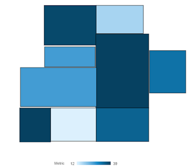
Here is a pictorial representation of Related datasets generated by different out of the box Machine algorithms in Oracle Data Visualization V4:


Different ML algorithms generate similar Related datasets and all of them can be clubbed into 8 datasets. Individual parameters and column names may change in dataset depending on the type of algorithm, but the functionality of dataset remains the same for ex: columns in Statistics dataset may change Linear Regression and Logistic Regression, but statistics dataset contains accuracy metrics of the model. Here is a brief description of each of these datasets:

1) Drivers: This dataset gives information on columns that are key determinants/drivers of the target column value. Train/Create model performs linear regression and identifies columns that take part in predicting the values for target column. Each of the identified columns are assigned coefficient and correlation values. Coefficient value talks about the weight-age given to that column in determining the target column value and correlation refers to the direction of relationship with target column i.e., if the target value increases or decreases with corresponding change in dependent column.

2) Residuals: This dataset also gives information on the quality of model prediction, Residuals in particular. Residual is the difference between the measured value and the predicted value of a regression model. This dataset gives an aggregated(sum) value of absolute difference between Actual and Predicted values for all the columns in dataset. This dataset is visualized using a bar graph in the Quality tab Linear Regression model Inspect menu.

3) CARTree: This dataset is a tabular representation of Decision Tree computed to predict the target column values. It contains columns that represent the conditions and criteria for conditions in decision tree, prediction for each group, prediction confidence. Inbuilt Tree Diagram visualization can be used to visualize this decision tree.

4) Confusion.Matrix: Confusion Matrix also known as error matrix is a specific table(pivot) layout that allows visualization of performance of an algorithm. Each row of the matrix represents instances of predicted class while each column represents instances in an actual class. This table reports the number of false positives, false negatives, true positives, and true negatives based on which precision, recall, F1 accuracy metrics are computed.

5) Hitmap: This dataset contains information on leaf nodes in the decision tree. Each row in the table represents a leaf node and it contains information the criteria/Branch-segment that leaf node represents, Segment Size, Confidence and Expected # of rows i.e., expected number of correct predictions = Segment Size * Confidence.

6) ClassificationReport: This dataset is a tabular representation of accuracy metrics for each distinct value of target column. For ex: if the target column can have two distinct values 'Yes' and 'No' , this dataset shows accuracy metrics like F1, Precision, Recall, Support(number of rows in Training dataset with this value) for each and every distinct value of Target column.

7) Summary: This dataset contains a summary of input and optional parameters to the model specified during model creation and contains details like Target name and Model name.

8) Statistics: This dataset contains metrics that quantify model accuracy. Depending on the algorithm/model that generates this dataset metrics present in the dataset will vary. Here is a list of metrics based on the model:

  • Linear Regression, CART numeric, Elastic Net Linear:
    • R-Square, R-Square Adjusted, Mean Absolute Error(MAE), Mean Squared Error(MSE), Relative Absolute Error(RAE), Related Squared Error(RSE), Root Mean Squared Error(RMSE)
  • CART(Classification And Regression Trees), Naive Bayes Classification, Neural Network, Support Vector Machine(SVM), Random Forest, Logistic Regression:
    • Accuracy, Total F1

Now you know what the Related datasets are and how they can be useful for fine tuning your Machine Learning model or for comparing two different models.

Are you an Oracle Analytics customer or user?

We want to hear your story!

Please voice your experience and provide feedback with a quick product review for Oracle Analytics Cloud!
 

.

Maps - How to extract a geoJSON from Oracle DB map theme for use in OracleDV


In this blog we will discuss about how to create a GeoJSON map layer from an existing Oracle DB map theme. This helps Oracle customers who have their maps/spatial data in Oracle Database and wants to leverage that investment in Oracle Analytics - Data Visualization. 

What is an Oracle Map Theme? Oracle Map Themes are also called Geometry Theme. A theme is a visual representation of a particular data layer. Using Oracle Map builder you can extract a GeoJSON from this Geometry theme. This geoJSON can be directly uploaded into Oracle Data Visualization as a custom map layer.

 Oracle DB Map Theme for a sample of congressional districts (preview on Oracle Map Builder):


Extracted map layer rendered in Oracle Data Visualization Map:

Detailed steps on how to do this conversion can be found in this document

High level steps:

1) Install Oracle Map Builder(If not installed already).
2) Connect to the Database Schema where the maps/Spatial data is present
3) Select the table that contains Geometry Theme data
4) Use Map Builder tools to extract this geometry table in to geoJSON.

Are you an Oracle Analytics customer or user?

We want to hear your story!

Please voice your experience and provide feedback with a quick product review for Oracle Analytics Cloud!


-

Maps - How to convert a Map Shapefile to geoJSON for use in Oracle DV

Have geographic map layer data sitting in a shapefile format and would like to visualize it in Oracle Data Visualization? In this blog we will discuss how to use Oracle tools to convert a shapefile into geoJSON format for use in Oracle Data Visualization.

Shapefile format is a digital vector storage format for storing geometric location and associated attribute information. The shapefile format can spatially describe vector features like points, lines, and polygons representing different kind of geographies.  File name extension of shapefiles is .shpMore information on shapefiles can be found here. 


GeoJSON is a format for encoding a variety of geographic data structures like maps of Cities, State, countries etc. Oracle DV supports custom map layers defined in GeoJSON formats.   

Using Oracle Map Builder you can convert shapefiles to geoJSON files. GeoJSON can be directly uploaded into OracleDV as a custom map layer and the data can be visualized directly on top of the Map layer. See detailed instructions here

Overview of steps involved:

1) Install Oracle Map Builder .
2) Use Export to JSON feature in Map Builder and use ShapefileSDP as source type and use the shape file to convert.
3) Choose appropriate key columns and SRID to do the conversion.

Are you an Oracle Analytics customer or user?

We want to hear your story!

Please voice your experience and provide feedback with a quick product review for Oracle Analytics Cloud!
 
.

Maps - How to convert an Image to geoJSON for use in Oracle DV


Many a time we would encounter images of a geographic layout(like a floor plan of a shopping mall, musuem, Airport or a demo hall etc) and wonder how great it would be to be able to visualize data with this layout as a map layer in OracleDV. Great news is this is possible! and in this blog we will discuss about how to convert an image to a geoJSON file format. Using a combination of Oracle tools users can convert image of a layout into geoJSON

Here is a snapshot that shows how a floor plan map layer extracted from an image looks like:
                                       
                                                             Floor Plan Image

                              
                                   Floor Plan Custom Map Layer extracted from Image
                           

One way to achieve this is using Oracle Map Builder and Oracle Map Editor tools. 

Step by step instructions on how to convert image to a map layer: Image to geoJSON Map Layer
 
Here is a high level view of steps involved in this process: 

1) Create a Base Map using the Image file received, using Oracle Map Builder tool. 
2) Create a GeoRaster theme using the Base Map using Map Builder tool
3) Create a Base Map based on the GeoRaster Theme using Map builder tool
4) Create a Geometry layer to show different regions on the map using Map Editor tool
5) Create a Theme(a database table) based on the Geometry Layer using Map Builder tool
6) Export the Theme to geoJSON using Oracle Map builder.

Are you an Oracle Analytics customer or user?

We want to hear your story!

Please voice your experience and provide feedback with a quick product review for Oracle Analytics Cloud!


-