Oracle Analytics Cloud supports advanced analytics functions with the single click of a mouse button, hiding all the underlying code & math required to support these. It supports capabilities like forecast, outliers identification, clusters computation, and trend-lines. Unlike writing a formula, this right click capability helps the users to quickly enrich their visualizations with advanced analytics based insights.
Advanced analytics capabilities can be added to charts in two different ways by the click of a mouse:
1) By right-clicking on the chart

2) or by visiting the bottom left Chart Properties pane :


Various properties of the forecast part can be controlled from the properties pane of the viz. Number of periods to be forecasted can be chosen by overriding the default. Confidence areas can be edited or turned off by setting the prediction interval. Eventually, the forecasting model used to calculate forecast can be chosen between these 3 options :
Choose the appropriate prediction interval to get an estimate of an interval in which a future observation will fall, with a certain probability, given what has already been observed.

The right-click option we describe here is the quick way to add a forecast to most of your analysis. If you wish to go deeper and persist the forecast to be reused in other visualizations, then you may as well create a custom calculation using the same forecast function. It provides with more control over the various options for the computation, here is the syntax
FORECAST(numeric_expr, series, output_column_name, options, runtime_binded_options)
numeric _expr : represents the metric to be forecasted.
series : is the time grain at which the forecast model is built.
dimension columns. this is the dimension grain you want to forecast on. If series is omitted, that is basically the grain of your data query.
output_column_name : is the output column. The valid values are
options : is a string list of name=value pairs each separated by ';'. The values can directly be hardcoded values, or they can refer to a column for example. In this case, put %1 ... %N, for the value and it will reference the same sequenced column in runtime_binded_options.
runtime_binded_options: is an optional comma separated list of runtime binded colums or literal expressions.
Example with ARIMA : In the example, model type used in ARIMA, no of periods to forecast is 6 while prediction interval is 70
FORECAST(
revenue,
(time_year, time_quarter),
'forecast',
'modelType=arima;numPeriods=6;predictionInterval=70;'
)
Example with ETS : In the example, model type used in ETS, no of periods to forecast is 6 while prediction interval is 70
FORECAST(
revenue,
(time_year, time_quarter),
'forecast',
'modelType=ETS;numPeriods=6;predictionInterval=70;'
)

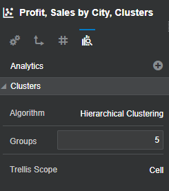
Properties of a Cluster calculation can be controlled from the properties pane, like number of clusters for exp. Choose the algorithm used for Clustering between K-means clustering and Hierarchical clustering.
a) K-means clustering: aims to partition n observations into k clusters in which each observation belongs to the cluster with the nearest mean, serving as a prototype of the cluster.
b) Hierarchical clustering: a hierarchy of clusters is built either by agglomerative (bottom-up) or a Divisive (top-down) approach.
A number of clusters can be chosen by entering an appropriate number.

As for other advanced analytics options, if you wish to dig deeper and have more control over how the cluster is being calculated, there is an option to create a calculated column using the cluster function. Here is the syntax
CLUSTER((dimension_expr1 , ... dimension_exprN), (expr1, ... exprN), output_column_name, options, runtime_binded_options)
dimension_expr : represents a list of dimensions , e.g. (productID, companyID), to be the individuals clustered.
expr represents : a list of attributes or measures that make up the 'space' (all the variables) that will be used to cluster the selected dimension_expr.
output_column_name : is the output column. The valid values are ''clusterId', 'clusterName', 'clusterDescription', 'clusterSize', 'distanceFromCenter', 'centers'.
options : is a string list of name=value pairs each separated by ';'. The values can directly be hardcoded values, or they can refer to a column for example. In this case, put %1 ... %N, for the value and it will reference the same sequenced column in runtime_binded_options.
runtime_binded_options: is an optional comma separated list of runtime binded colums or literal expressions.
Example with Clusters : Here the algorithm used is k-means with no of clusters - 5 without the usage of random seed.
CLUSTER((product, company), (billed_quantity, revenue), 'clusterName', 'algorithm=k-means;numClusters=5;maxIter=%2;useRandomSeed=FALSE;enablePartitioning=TRUE')

Outliers calculation also offers option to choose between algorithms K-means and Hierarchical to be computed.

Right-click option is a quick way to add outliers to your analysis. If you wish to dig deeper and have more control over how the outlier is being calculated, there is an option to create a calculated column using the outlier function. Here is the syntax
OUTLIER((dimension_expr1 , ... dimension_exprN), (expr1, ... exprN), output_column_name, options, [runtime_binded_options])
dimension_expr: represents a list of dimensions , e.g. (Product, Department)
expr: represents: a list of dimension attributes or measures to be used find outlier's.
options : is a string list of name=value pairs each separated by ';'. The values can directly be hardcoded values, or they can refer to a column for example. In this case, put %1 ... %N, for the value and it will reference the same sequenced column in runtime_binded_options.
runtime_binded_options: is an optional comma separated list of runtime binded colums or literal expressions.
Example with Outliers : Here the algorithm used is mvoutlier.
OUTLIER((product, company), (billed_quantity, revenue), 'isOutlier', 'algorithm=mvoutlier')

Configuration options of the trendline can be controlled in the options pane. The method for
the trend line has 3 options
Confidence Interval A confidence interval is a range of values, derived from sample statistics, that is likely to contain the value of an unknown population parameter. Because of their random nature, it is unlikely that two samples from a given population will yield identical confidence intervals.

Trendline can also be calculated in a custom calculation :
TRENDLINE(numeric_expr, ([series]) BY ([partitionBy]), model_type, result_type)
numeric_expr: represents the data to trend. This is the Y-axis. This is usually a measure column.
series: is the X-axis. It is a list of numeric or time dimension attribute columns.
partitionBY: is a list of dimension attribute columns that are in the view but not on the X-axis.
model_type: is one of the following ('LINEAR', 'EXPONENTIAL').
result_type: is one of the following ('VALUE', 'MODEL'). 'VALUE' will return all the regression Y values given X in the fit. 'MODEL' will return all the parameters in a JSON format string.
Example with Trendline : Trend of revenue by by product using linear regression.
TRENDLINE(revenue, (calendar_year, calendar_quarter, calendar_month) BY (product), 'LINEAR', 'VALUE')
Here is an example where the reference line is added on a report where we have Sales by Month. The reference is plotted on the average value of the Sales.

The other method to draw a reference line is Band. The band provides 2 lines with a range of reference. The function can be chosen between Custom and Standard Deviation, while the upper limit and lower limit of the reference line can be chosen between Average, Maximum, Minimum, etc. For example, if we are analyzing sales by month and we have a reference band plotted from Average to maximum, it would be easy to find out, in which months the sales were falling in the above average, below the maximum band.

The function can also be chosen as Standard Deviation and you have an option to select the value of 1,2 or 3. If you choose 1, then the band is drawn in such a way that 68% of values lie within the band. If you choose 2, then 95% of the value lies and for 3, 99.7% of values lie within the band.

If you like to see a live project which showcases these advanced capabilities, please visit our Sandbox environments here
Oracle Analytics cloud offers a pretty user-friendly method to leverage advanced analytics functions on a chart with a single mouse click. Having advanced analytical functions like Forecast, cluster and outliers provide a strong capability to business users to have better insights into data.
Advanced analytics capabilities can be added to charts in two different ways by the click of a mouse:
1) By right-clicking on the chart

2) or by visiting the bottom left Chart Properties pane :

Forecast
Forecasting is the process of making predictions of the future, based on past and present data and most commonly by analysis of trends. In this example, we have a report showing Sales by Month and let's forecast Sales by adding it to the chart. The Sales line extends to show forecast with distinguishable color to it.

Various properties of the forecast part can be controlled from the properties pane of the viz. Number of periods to be forecasted can be chosen by overriding the default. Confidence areas can be edited or turned off by setting the prediction interval. Eventually, the forecasting model used to calculate forecast can be chosen between these 3 options :
- ARIMA (Moving Average, default): assumes that overall past data is a reliable base to explain & project the future
- Seasonal ARIMA: if you find a regular pattern of changes that repeats over time periods, then choose Seasonal Arima.
- ETS : Exponential Triple Smoothing is often used in analysis of time series data.
Choose the appropriate prediction interval to get an estimate of an interval in which a future observation will fall, with a certain probability, given what has already been observed.

The right-click option we describe here is the quick way to add a forecast to most of your analysis. If you wish to go deeper and persist the forecast to be reused in other visualizations, then you may as well create a custom calculation using the same forecast function. It provides with more control over the various options for the computation, here is the syntax
FORECAST(numeric_expr, series, output_column_name, options, runtime_binded_options)
numeric _expr : represents the metric to be forecasted.
series : is the time grain at which the forecast model is built.
dimension columns. this is the dimension grain you want to forecast on. If series is omitted, that is basically the grain of your data query.
output_column_name : is the output column. The valid values are
- 'forecast' : forecast value
- 'low', : value of the confidence interval low-bound
- 'high',: value of the confidence interval high-bound,
- 'predictionInterval' : value of the confidence prediction interval used for this forecast
options : is a string list of name=value pairs each separated by ';'. The values can directly be hardcoded values, or they can refer to a column for example. In this case, put %1 ... %N, for the value and it will reference the same sequenced column in runtime_binded_options.
runtime_binded_options: is an optional comma separated list of runtime binded colums or literal expressions.
Example with ARIMA : In the example, model type used in ARIMA, no of periods to forecast is 6 while prediction interval is 70
FORECAST(
revenue,
(time_year, time_quarter),
'forecast',
'modelType=arima;numPeriods=6;predictionInterval=70;'
)
Example with ETS : In the example, model type used in ETS, no of periods to forecast is 6 while prediction interval is 70
FORECAST(
revenue,
(time_year, time_quarter),
'forecast',
'modelType=ETS;numPeriods=6;predictionInterval=70;'
)
Clusters
Cluster analysis or clustering is the task of grouping a set of objects in such a way that objects in the same group are show a coherence and maximal proximity to each other than to those in other groups. In this example, we have a scatter plot where profit and Sales are plotted against each other with all the scatter dots representing cities. The colors of the dots represent the various clusters that they are grouped into.
Properties of a Cluster calculation can be controlled from the properties pane, like number of clusters for exp. Choose the algorithm used for Clustering between K-means clustering and Hierarchical clustering.
a) K-means clustering: aims to partition n observations into k clusters in which each observation belongs to the cluster with the nearest mean, serving as a prototype of the cluster.
b) Hierarchical clustering: a hierarchy of clusters is built either by agglomerative (bottom-up) or a Divisive (top-down) approach.
A number of clusters can be chosen by entering an appropriate number.
As for other advanced analytics options, if you wish to dig deeper and have more control over how the cluster is being calculated, there is an option to create a calculated column using the cluster function. Here is the syntax
CLUSTER((dimension_expr1 , ... dimension_exprN), (expr1, ... exprN), output_column_name, options, runtime_binded_options)
dimension_expr : represents a list of dimensions , e.g. (productID, companyID), to be the individuals clustered.
expr represents : a list of attributes or measures that make up the 'space' (all the variables) that will be used to cluster the selected dimension_expr.
output_column_name : is the output column. The valid values are ''clusterId', 'clusterName', 'clusterDescription', 'clusterSize', 'distanceFromCenter', 'centers'.
options : is a string list of name=value pairs each separated by ';'. The values can directly be hardcoded values, or they can refer to a column for example. In this case, put %1 ... %N, for the value and it will reference the same sequenced column in runtime_binded_options.
runtime_binded_options: is an optional comma separated list of runtime binded colums or literal expressions.
Example with Clusters : Here the algorithm used is k-means with no of clusters - 5 without the usage of random seed.
CLUSTER((product, company), (billed_quantity, revenue), 'clusterName', 'algorithm=k-means;numClusters=5;maxIter=%2;useRandomSeed=FALSE;enablePartitioning=TRUE')
Outliers
Outliers are data records that are located the furthest away from the average expectation of individuals values. For example extreme values that deviate the most from other observations on data. They may indicate variability in measurement, experimental errors or a novelty. To the same report where the clusters are added, outliers are added and depicted as different shapes. Scatter dots represented by circles are outliers while the ones represented by squares are non-outliers.
Outliers calculation also offers option to choose between algorithms K-means and Hierarchical to be computed.

Right-click option is a quick way to add outliers to your analysis. If you wish to dig deeper and have more control over how the outlier is being calculated, there is an option to create a calculated column using the outlier function. Here is the syntax
OUTLIER((dimension_expr1 , ... dimension_exprN), (expr1, ... exprN), output_column_name, options, [runtime_binded_options])
dimension_expr: represents a list of dimensions , e.g. (Product, Department)
expr: represents: a list of dimension attributes or measures to be used find outlier's.
options : is a string list of name=value pairs each separated by ';'. The values can directly be hardcoded values, or they can refer to a column for example. In this case, put %1 ... %N, for the value and it will reference the same sequenced column in runtime_binded_options.
runtime_binded_options: is an optional comma separated list of runtime binded colums or literal expressions.
Example with Outliers : Here the algorithm used is mvoutlier.
OUTLIER((product, company), (billed_quantity, revenue), 'isOutlier', 'algorithm=mvoutlier')
Trendlines
Similar to adding a forecast for your metric, you can measure the trend of your metric by adding a trend line which indicates a general course of the tendency of the metric in question. A trendline is a straight line connecting a number of points on a graph. It is used to analyze the specific direction of a group of values set in a presentation. In this example, we have Sales by Month and the trendline shows that Sales is on the incline.

Configuration options of the trendline can be controlled in the options pane. The method for
the trend line has 3 options
- Linear: A linear trend line is a best fit straight line with linear data sets. Your data is linear if the patter in its data points resembles a line. A linear trend line shows that your metric is increasing or decreasing at a steady rate.
- Polynomial: A polynomial trendline involves an equation with several factors of the main X value with various exponent degrees (level 2 = x square, 3=x cubic power...). The result is a curved line that may better fit your data when data fluctuates up and down. It is useful, for example, for understanding gains and losses over a large data set. The order of the polynomial can be determined by the number of fluctuations in the data or by how many bends (hills and valleys) appear in the curve.
- Exponential: An exponential trendline is a curved line that is most useful when data values rise or fall at increasingly higher rates. You cannot create an exponential trendline if your data contains zero or negative values.
Confidence Interval A confidence interval is a range of values, derived from sample statistics, that is likely to contain the value of an unknown population parameter. Because of their random nature, it is unlikely that two samples from a given population will yield identical confidence intervals.

Trendline can also be calculated in a custom calculation :
TRENDLINE(numeric_expr, ([series]) BY ([partitionBy]), model_type, result_type)
numeric_expr: represents the data to trend. This is the Y-axis. This is usually a measure column.
series: is the X-axis. It is a list of numeric or time dimension attribute columns.
partitionBY: is a list of dimension attribute columns that are in the view but not on the X-axis.
model_type: is one of the following ('LINEAR', 'EXPONENTIAL').
result_type: is one of the following ('VALUE', 'MODEL'). 'VALUE' will return all the regression Y values given X in the fit. 'MODEL' will return all the parameters in a JSON format string.
Example with Trendline : Trend of revenue by by product using linear regression.
TRENDLINE(revenue, (calendar_year, calendar_quarter, calendar_month) BY (product), 'LINEAR', 'VALUE')
Reference Lines
Reference lines are vertical or horizontal lines in a graph, corresponding with user-defined values on the x-axis and y-axis respectively.
By default the reference line is of type - line and the method chosen for the computation of the line can be chosen from the various options like Average, Minimum, Maximum, etc. For example, In an airline industry, if passenger turnout is plotted wrt to time, the reference would be able to guide users to know whether the passenger turnout for a particular month is above or below average.Here is an example where the reference line is added on a report where we have Sales by Month. The reference is plotted on the average value of the Sales.

The other method to draw a reference line is Band. The band provides 2 lines with a range of reference. The function can be chosen between Custom and Standard Deviation, while the upper limit and lower limit of the reference line can be chosen between Average, Maximum, Minimum, etc. For example, if we are analyzing sales by month and we have a reference band plotted from Average to maximum, it would be easy to find out, in which months the sales were falling in the above average, below the maximum band.

The function can also be chosen as Standard Deviation and you have an option to select the value of 1,2 or 3. If you choose 1, then the band is drawn in such a way that 68% of values lie within the band. If you choose 2, then 95% of the value lies and for 3, 99.7% of values lie within the band.

If you like to see a live project which showcases these advanced capabilities, please visit our Sandbox environments here
Oracle Analytics cloud offers a pretty user-friendly method to leverage advanced analytics functions on a chart with a single mouse click. Having advanced analytical functions like Forecast, cluster and outliers provide a strong capability to business users to have better insights into data.
Are you an Oracle Analytics customer
or user?
We want to hear your story!
Please voice your experience and provide feedback
with a quick product review for Oracle Analytics Cloud!


